Working with Multinomial Proportions
MPA 6010
Ani Ruhil
Agenda
Hypothesis tests with Multinomial Proportions
Hypothesis tests for one-group proportions
Hypothesis tests for two-group proportions
Multinomial data
Data from a single population are often categorical
For example,
market shares of Internet Explorer; Firefox; Safari; Chrome
voters identifying themselves as Democrats; Independents; Republicans
wealth classified as Poor; Low Income; Middle Income; High Income; Rich
Number of Gold, Silver, Bronze medals at the Olympic games
Individuals who Strongly Disagree, Neither Disagree nor Agree, or Strongly Agree with a statement
The hypothesis test then involves looking at the sample proportions vis-a-vis those we suspect/expect to be true for the population
Mechanics of Hypothesis Test for Multinomial Population
\(H_{0}: P_{a} = x\%, P_{b} = y\%, P_{c} = z\%\)
\(H_{1}:P_{a} \neq x\%, P_{b} \neq y\%, P_{c} \neq z\%\)
Test Statistic is
$$\chi^{2} = \sum ^{k} _{i=1} \dfrac{(f_{i} - e_{i})^{2}}{e_{i}}$$
where ... \(f_{i}=\) Observed frequency, \(e_{i}=\) Expected frequency, and \(k=\) Number of categories
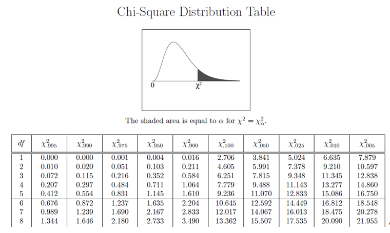
\(\chi^{2} \sim\) with \(df=k-1\) if \(e_{i} \geq 5\) for all categories
Reject \(H_{0}\) if \(p-value \leq \alpha\) or, alternatively, Reject \(H_{0}\) if Calculated \(\chi^{2} \geq\) Critical \(\chi^{2}\)
Example 1
We have four health campaigns that air. Null hypothesis is that each is recalled by identical proportion of viewers.
\(H_{0}:P_{a}=0.25; P_{b}=0.25; P_{c}=0.25; P_{d}=0.25\) and \(H_{1}:\) Proportions are different
\(e_{a} = 0.25(300)=75; e_{b} = 0.25(300)=75;\); \(e_{c} = 0.25(300)=75; e_{d} = 0.25(300)=75\)
| Campaign | \(f_{i}\) | \(e_{i}\) | \((f_{i}-e_{i})\) | \((f_{i}-e_{i})^{2}\) | \((f_{i}-e_{i})^{2}/{e_{i}}\) |
|---|---|---|---|---|---|
| a | 85 | 75 | 10 | 100 | 1.3333 |
| b | 95 | 75 | 20 | 400 | 5.3333 |
| c | 50 | 75 | -25 | 625 | 8.3333 |
| d | 70 | 75 | -5 | 25 | 0.3333 |
| Total | 300 | 300 | 15.3333 |
\(\chi^{2}_{df=3} = 15.3333\)
\(p-value < 0.005\); Reject \(H_{0}\); The proportions are different and so the health campaigns are not all equally effective
Example 2
M&M/MARS' manufacturing plants have different color mixes, ands these change over time. The 1997 color mix are in parentheses below. How does the actual distribution of colors in 506 M&Ms match that prescribed by the company?
| Colors | \(f_{i}\) | \(e_{i}\) | \((f_{i}-e_{i})\) | \((f_{i}-e_{i})^{2}\) | \((f_{i}-e_{i})^{2}/{e_{i}}\) |
|---|---|---|---|---|---|
| Blue (10%) | 38 | 50.6 | -12.6 | 158.76 | 3.1375 |
| Brown (30%) | 177 | 151.8 | 25.2 | 635.04 | 4.1834 |
| Green (10%) | 36 | 50.6 | -14.6 | 213.16 | 4.2126 |
| Orange (10%) | 41 | 50.6 | -9.6 | 92.16 | 1.8213 |
| Red (20%) | 79 | 101.2 | -22.2 | 492.84 | 4.8700 |
| Yellow (20%) | 135 | 101.2 | 33.8 | 1142.44 | 11.2889 |
| Total | 506 | 29.5138 |
\(\chi^{2}_{df=5} = 29.5138\), and the \(p-value < 0.005\); Reject \(H_{0}\); Data do not reflect 1997 color percentages
The Chi-Squared test of Independence/Association
\(\chi^{2}\) tests can also be used to test independence of two variables
For e.g., look at the following contingency table/crosstabulation
| Gender | Light | Regular | Dark | Total |
|---|---|---|---|---|
| Male | 20 | 40 | 20 | 80 |
| Female | 30 | 30 | 10 | 70 |
| Total | 50 | 70 | 30 | 150 |
Research Question: Are coffee preferences independent of gender (i.e., is there any association between coffee preferences and gender)?
\(H_{0}:\) Coffee preference is independent of gender
\(H_{1}:\) Coffee preference is not independent of gender
For each cell in the contingency table, calculate
$$e_{ij} = \dfrac{\text{Row } i \text{ Total} \times \text{Column } j \text{ Total}}{\text{Sample Size}}$$
\(e_{11}=\dfrac{(80)(50)}{150}=\dfrac{4000}{150}=26.67\)
\(e_{12}=\dfrac{(80)(70)}{150}=\dfrac{5600}{150}=37.33\)
\(e_{13}=\dfrac{(80)(30)}{150}=\dfrac{2400}{150}=16.00\)
\(e_{21}=\dfrac{(70)(50)}{150}=\dfrac{3500}{150}=23.33\)
\(e_{22}=\dfrac{(70)(70)}{150}=\dfrac{4900}{150}=32.67\)
\(e_{23}=\dfrac{(70)(30)}{150}=\dfrac{2100}{150}=14.00\)
Calculate, for each cell in the contingency table, \(\dfrac{(f_{ij}-e_{ij})^{2}}{e_{ij}}\)
Add the resulting value over all cells
This yields $$\chi^{2} = \sum_{i} \sum_{j} \dfrac{(f_{ij} - e_{ij})^{2}}{e_{ij}}$$
\(\chi^{2} \sim df=(r-1)(c-1)\) where ... \(r=\) number of rows, and \(c=\) number of columns
Why are \(df = (r-1)(c-1)\) ?
Degrees of freedom: \(df = (r-1)(c-1)\)
| Gender | Light | Regular | Dark | Total |
|---|---|---|---|---|
| Male | 20 | 40 | ? | 80 |
| Female | ? | 30 | 10 | 70 |
| Total | 50 | 70 | 30 | 150 |
Completing the Coffee vs. Gender Example
| Gender | \(f_{i}\) | \(e_{i}\) | \((f_{i}-e_{i})\) | \((f_{i}-e_{i})^{2}\) | \((f_{i}-e_{i})^{2}/{e_{i}}\) |
|---|---|---|---|---|---|
| Male | 20 | 26.67 | -6.67 | 44.49 | 1.67 |
| Male | 40 | 37.33 | 2.67 | 7.13 | 0.19 |
| Male | 20 | 16.00 | 4.00 | 16.00 | 1.00 |
| Female | 30 | 23.33 | 6.67 | 44.49 | 1.91 |
| Female | 30 | 32.67 | -2.67 | 7.13 | 0.22 |
| Female | 10 | 14.00 | -4.00 | 16.00 | 1.14 |
| \(\chi^{2}\) | 6.13 |
\(df=(r-1)(c-1)=(2-1)(3-1)=(1)(2)=2\)
\(p-value < 0.05\); Reject \(H_{0}\)
Coffee preferences and gender are not independent
Another Example
WA's Public Interest Research Group (PIRG) found in its recent study that 46% of full-time college students work 25 or more hours per week. A sample of 200 included 90 who worked 1-15 hours per week, 60 who worked 16-24 hours per week, and 50 who worked 25-34 hours per week. Students were also asked if their work had a positive, negative, or no effect on their grades. Use \(\alpha = 0.01\)
| Hours Worked/Week | Positive | None | Negative | Total |
|---|---|---|---|---|
| 1-15 hours | 26.00 | 50.00 | 14.00 | 90.00 |
| 16-24 hours | 16.00 | 27.00 | 17.00 | 60.00 |
| 25-34 hours | 11.00 | 19.00 | 20.00 | 50.00 |
| Total | 53.00 | 96.00 | 51.00 | 200.00 |
Calculated Expected Frequencies
| Hours Worked/Week | Positive | None | Negative | Total |
|---|---|---|---|---|
| 1-15 hours | 23.85 | 43.20 | 22.95 | 90.00 |
| 16-24 hours | 15.90 | 28.80 | 15.30 | 60.00 |
| 25-34 hours | 13.25 | 24.00 | 12.75 | 49.95 |
| Total | 53.00 | 96.00 | 51.00 | 200.00 |
| 1-15 hours | 0.19 | 1.07 | 3.49 | 4.75 |
| 16-24 hours | 0.00 | 0.11 | 0.19 | 0.30 |
| 25-34 hours | 0.38 | 1.04 | 4.12 | 5.54 |
| \(\chi^{2}_{df=4}\) | 10.59 |
What is your decision? To Reject or not to Reject?
Do More Working Hours Mean Poorer Grades?
How would you answer this question? Column vs Row Percentages
| Hours/Week | Positive | None | Negative | Total |
|---|---|---|---|---|
| 1-15 hours | 28.89% | 55.56% | 15.56% | 100.00% |
| 16-24 hours | 26.67% | 45.00% | 28.33% | 100.00% |
| 25-34 hours | 22.00% | 38.00% | 40.00% | 100.00% |
| Hours/Week | Positive | None | Negative | |
|---|---|---|---|---|
| 1-15 hours | 49.05% | 52.08% | 27.45% | |
| 16-24 hours | 30.18% | 28.12% | 33.33% | |
| 25-34 hours | 20.75% | 19.79% | 39.21% | |
| Total | 100% | 100% | 100% |
As a student's hours worked per week increase, the negative effect on his/her grades increases
A Cautionary Tale
Table (a)
| Hours worked/week | Positive | None | Negative | Total |
|---|---|---|---|---|
| 1-15 hours | 26 | 50 | 14 | 90 |
| 16-24 hours | 16 | 27 | 17 | 60 |
| 25-34 hours | 11 | 19 | 20 | 50 |
| Total | 53 | 96 | 51 | 200 |
Table (b)
| Hours worked/week | Positive | None | Negative | Total |
|---|---|---|---|---|
| 1-15 hours | 260 | 500 | 140 | 900 |
| 16-24 hours | 160 | 270 | 170 | 600 |
| 25-34 hours | 110 | 190 | 200 | 500 |
| Total | 530 | 960 | 510 | 2000 |
| Hours | Positive | None | Negative | Total |
|---|---|---|---|---|
| 1-15 hours | 260 | 500 | 140 | 900 |
| 16-24 hours | 160 | 270 | 170 | 600 |
| 25-34 hours | 110 | 190 | 200 | 500 |
| Total | 530 | 960 | 510 | 2000 |
| Hours | Positive | None | Negative | Total |
|---|---|---|---|---|
| 1-15 hours | 238.50 | 432.00 | 229.50 | 900 |
| 16-24 hours | 159.00 | 288.00 | 153.00 | 600 |
| 25-34 hours | 132.50 | 240.00 | 127.50 | 500 |
| Total | 530 | 960 | 510 | 2000 |
| Hours worked/week | Positive | None | Negative | Total |
|---|---|---|---|---|
| 1-15 hours | 1.94 | 10.70 | 34.90 | 47.54 |
| 16-24 hours | 0.01 | 1.13 | 1.89 | 3.02 |
| 25-34 hours | 3.82 | 10.42 | 41.23 | 55.46 |
| \(\chi^{2}_{df=4}\) | 106.03 |
Large samples will typically yield statistically significant results and so one also needs to focus on substantive significance -- how large an effect does the independent variable have? See here for a beautiful piece on this issue. This is most important for policy analysis and program evaluation in our fields
Distance to a Hospital and Visit Frequency
Using the data given below, test for an association between the proximity of residence to the hospital and the frequency of visits to the hospital's ER unit.
| Frequency of Visits | Close | Medium | Far | Total |
|---|---|---|---|---|
| Low | 1000 | 1030 | 1050 | 3080 |
| Medium | 525 | 520 | 515 | 1560 |
| High | 475 | 450 | 435 | 1360 |
| Total | 2000 | 2000 | 2000 | 6000 |
Calculating the expected frequencies ...
| Frequency of Visits | Close | Medium | Far |
|---|---|---|---|
| Low | (3080 x 2000)/6000 | (3080 x 2000) /6000 | (3080 x 2000)/ 6000 |
| Medium | (1560 x 2000)/6000 | (1560 x 2000) /6000 | (1560 x 2000)/ 6000 |
| High | (1360 x 2000)/6000 | (1360 x 2000) /6000 | (1360 x 2000)/ 6000 |
Use this online \(\chi^2\) calculator
Fisher's Exact Test
The \(\chi^2\) test assumes that
(1) At least 80% of the cells in the table have expected frequencies \(\geq 5\), and
(2) No cell in the table has an expected frequency \(< 1\)
If this assumption is violated, you can try to collapse some categories (for e.g., if the categories are 0, 1-2, 3-4, 5-6, and 7 or more, and the 7 or more category has an expected frequency \(< 1\), you can collapse it into the preceding category to generate a new category called 5 or more. This collapsing has to be defensible.
You can also collapse Strongly Disagree and Agree Somewhat into Agree, Strongly Disagree and Agree Somewhat to generate a three-point classification of 'Disagree', 'Neither Disagree nor Agree', 'Agree', and so on. Again, the collapsing has to be defensible.
Else you can rely on Fisher's Exact Test, provided you have small samples and or a powerful computer
How does Fisher's Exact Test Work
| Therapy | Patient Improves | Patient does not improve | Total |
|---|---|---|---|
| Did pre-operative PT | 15 | 6 | 21 |
| Did not do pre-operative PT | 7 | 322 | 329 |
| Total | 22 | 328 | 350 |
Involves calculating the probability of ending up with the observed frequencies as recorded. Computationally intensive because it involves calculating, under the assumption that \(H_0\) is true, all possible \(2\times2\) tables that would yield the same row and column totals.
\(p-value = \dfrac{(a+b)!(c+d)!(a+c)!(b+d)!}{n!a!b!c!d!}\)
In this example the ensuing \(p-value = 2.2e-16\); so we reject \(H_0\). The patient improving is not independent of whether or not the patient was given pre-operative physical therapy.
See here for a wonderful example
The online calculator for Fisher's exact test can be found here
Hypothesis tests with proportions
One-Group Hypothesis Tests with \(z\)
- Lower Tail Test \(H_{0}: p \geq p_{0}; H_{1}: p < p_{0}\)
- Upper Tail Test \(H_{0}: p \leq p_{0}; H_{1}: p > p_{0}\)
- Two Tailed Test \(H_{0}: p = p_{0}; H_{1}: p \neq p_{0}\)
Sample standard deviation \(s = \sqrt{p_0 \times \left( 1 - p_0 \right)}\) and Standard Error of \(\bar{p}= s_{\bar{p}} = \dfrac{s}{\sqrt{n}}\)
Test Statistic is \(z=\dfrac{\bar{p}-p_{0}}{s_{\bar{p}}}\) and \(df = n-1\)
Confidence Intervals calculated as: \(\bar{p} \pm z_{\alpha/2} (\bar{s}_{\bar{p}})\) and adjusted with a continuity correction of \(\pm \dfrac{0.5}{n}\), with \(\bar{s}_{\bar{p}} = \dfrac{\sqrt{ \bar{p} \times (1 - \bar{p}) }}{\sqrt{n}}\)
Sample size needed calculated as before except the suspected standard deviation is typically set to \(0.5\) because
This yields the largest \(s\) ... \(\sqrt{0.5 \times (1 - 0.5)} = 0.5\) while \(\sqrt{0.1 \times (1 - 0.1)} = 0.3\)
Assuming a 50:50 split in the proportion is a good start unless we can assume otherwise
An Example
Consumer Reports study done in 2010 finds 64% of shoppers think national brands as good as generics. In January of 2019 Heinz asks this question of 100 shoppers and find 52% say generics are as good as national brands. Have consumer preferences changed?
Given \(p_{0}=0.64; n=100; \bar{p}=0.52\); \(H_{0}: p = 0.64; H_{1}: p \neq 0.64\)
$$\sigma_{\bar{p}}={\sqrt{\dfrac{p_{0}(1-p_{0})}{n}}}={\sqrt{\dfrac{0.64(0.36)}{100}}}=0.048$$
$$z=\dfrac{\bar{p}-p_{0}}{\sigma_{\bar{p}}}=\dfrac{0.52-0.64}{0.048}=\dfrac{-0.12}{0.48}=-2.50$$
\(p-value\) is thus 0.0124 and with \(\alpha = 0.05\), we can reject the null hypothesis; consumer preferences appear to have changed
Testing via the online calculator
Another Example
Census Bureau found in 1990 that 24% of those who moved residences did so to be closer to work. In 2010, 90 out of a random sample of 300 movers said so as well. Are more people moving to be closer to work in 2010 than did so in 1990?
Given \(p_{0}=0.24; n=300; \bar{p}=\dfrac{90}{300}=0.30\); \(H_{0}: p \leq 0.24; H_{1}: p > 0.24\)
$$\sigma_{\bar{p}}={\sqrt{\dfrac{p_{0}(1-p_{0})}{n}}}={\sqrt{\dfrac{0.24(0.76)}{300}}}=0.0246$$
$$z=\dfrac{\bar{p}-p_{0}}{\sigma_{\bar{p}}}=\dfrac{0.30-0.24}{0.0246}=\dfrac{0.06}{0.0246}=2.439024$$
\(p-value\) is 0.007363495 and hence with \(\alpha = 0.05\) we can easily reject the null hypothesis, concluding that compared with the 1990 Census, by 2010 more people were relocating to be closer to work
Yet another problem
After a massive inventory the Athens Public Library finds 12% of its books missing. They institute anti-theft measures and after a year, draw a sample of 200 books to see how many are missing and find they cannot locate 14 books. Have the new measures reduced theft?
\(H_0: p \geq 0.12\); \(H_1: p < 0.12\)
\(\bar{p} = \dfrac{14}{200} = 0.07\)
\(s = \sqrt{p_0 \times (1 - p_0)} = \sqrt{0.12 \times (1 - 0.12)} = \sqrt{0.12 \times 0.88} = 0.3249\)
\(s_{\bar{p}} = \dfrac{s}{\sqrt{n}} = \dfrac{0.3249}{\sqrt{200}} = 0.0229\)
\(z = \dfrac{\bar{p} - p_0}{s_{\bar{p}}} = \dfrac{0.07 - 0.12}{0.0229} = \dfrac{-0.05}{0.0229} = -2.1834\)
\(p-value = 0.015\) and so with \(\alpha = 0.05\) we reject \(H_0\); the data suggest that the measures have reduced thefts
What if you had used \(\alpha = 0.01\)? Would your conclusion have changed?
Two proportions
Two-Group Hypothesis Tests with z
Two groups so two proportions ... \(p_{1}; p_{2}\)
With \(n_{1}\) and \(n_{2}\), we have two sample proportions \(\bar{p_{1}}\) and \(\bar{p_{2}}\)
Point Estimate of the difference between the two groups is thus \(\bar{p_{1}} - \bar{p_{2}}\)
Standard deviation for each group is \(s_1 =\sqrt{\bar{p_1} \left(1-\bar{p_1} \right)}\) and \(s_2 =\sqrt{\bar{p_2} \left(1-\bar{p_2} \right)}\)
Standard error for each group is \(s_{\bar{p_1}} = \dfrac{s_1}{\sqrt{n_1}}\) and \(s_{\bar{p_2}} = \dfrac{s_2}{\sqrt{n_2}}\)
The overall standard error for both groups is \(s_{\bar{p_1} - \bar{p_2} } = \sqrt{\left( s_{\bar{p_1}} \right)^2 + \left(s_{\bar{p_2}} \right)^2 }\)
Distribution of the test statistic is \(N()\) if \(n_{1}p_{1}, n_{1}(1-p_{1}), n_{2}p_{2}, n_2(1-p_{2})\) are all \(\geq 5\)
Degrees of freedom now are \(df= n_1 + n_2 - 2\)
Interval Estimate is given by \(\bar{p_{1}} - \bar{p_{2}} \pm z_{\alpha/2} \left( s_{\bar{p_{1}} - \bar{p_{2}}} \right)\)
Hypothesis tests about \(p_{1}-p_{2} \cdots\)
- \(H_{0}:p_{1}-p_{2} \geq 0; H_{1}:p_{1}-p_{2} < 0\)
- \(H_{0}:p_{1}-p_{2} \leq 0; H_{1}:p_{1}-p_{2} > 0\)
- \(H_{0}:p_{1}-p_{2}=0; H_{1}:p_{1}-p_{2} \neq 0\)
Assuming \(H_{0}\) is true is equivalent to saying \(p_{1}=p_{2}=p\)
Testing via the online calculator
An Example with message recall
In a test of two anti-tobacco television commercials, random sample of television viewers were asked to recall the primary message in each. Let \(1=\) Commercial A and \(2 =\) Commercial B. Given \(n_1=150; n_2=200\) and that the number recalling the primary message were 63 and 60, respectively. Test the hypothesis of no difference in recall.
$$H_{0}:p_{1}-p_{2}=0; H_{1}:p_{1}-p_{2} \neq 0$$
$$\bar{p_{1}}=\dfrac{63}{150}=0.42; \bar{p_{2}}=\dfrac{60}{200}=0.30; df=n_1 + n_2 - 2 = 150+200-2=348$$
$$s_1 =\sqrt{\bar{p_1} \left(1-\bar{p_1} \right)} = \sqrt{ 0.42 \times (1 - 0.42) } = 0.4935$$
$$s_2 =\sqrt{\bar{p_2} \left(1-\bar{p_2} \right)} = \sqrt{ 0.30 \times (1 - 0.30) } = 0.4582$$
$$s_{\bar{p_1}} = \dfrac{s_1}{\sqrt{n_1}} = \dfrac{0.4935}{\sqrt{150}} = 0.0402; s_{\bar{p_2}} = \dfrac{s_2}{\sqrt{n_2}} = \dfrac{0.4582}{\sqrt{200}} = 0.0324$$
$$s_{\bar{p_1} - \bar{p_2} } = \sqrt{ \left( s_{\bar{p_1}} \right)^2 + \left(s_{\bar{p_2}} \right)^2 } = \sqrt{(0.0402)^2 + (0.0324)^2} = 0.0517$$
$$z=\dfrac{\bar{p_{1}} - \bar{p_{2}}}{s_{\bar{p_1} - \bar{p_2} }} =\dfrac{0.42-0.30}{0.0517} = \dfrac{0.12}{0.0517} = 2.3206$$
\(p-value = 0.0209\) so, we reject \(H_{0}\)}; Recall rates seem to differ across commercials
95% CI is \(\bar{p_{1}} - \bar{p_{2}} \pm z_{\alpha/2; df} ( s_{\bar{p_1} - \bar{p_2} }) = 0.12 \pm 1.967 (0.0517) = (0.0183; 0.2216) \cdots\) does not include \(H_0\) value of 0
What if we used \(\alpha=0.01\)? Would the conclusion change?
An Example with Helmet Laws
The Wisconsin legislature is considering a mandatory motorcycle helmet law. What legislators don't know is whether the law would encourage more people to use helmets. A Senator tells you that Minnesota has a similar law in use and so you conduct a random survey of registered motorcycle riders in each state. The results are given below:
| Minnesota | Wisconsin | |
|---|---|---|
| Sample Size | 75 | 110 |
| Number using helmets | 37 | 28 |
Setup the correct hypotheses
Using \(\alpha=0.01\), carry out the test
State the conclusion of your hypothesis test
What if the numbers using seat belts were 37 and 50, respectively?
Another Example: Racial Discrimination
The City Attorney for Columbus (OH) is gathering data for a racial discrimination lawsuit. When she asks 500 Latino residents of the city if they feel the city is racially biased, 354 reply in the affirmative. When she asks 300 non-Latino White residents the same question, 104 respond in the affirmative. Do these data suggest the Latinos perceive racial bias differently than do non-Latino-Whites?
Setup the correct hypotheses
Using \(\alpha=0.05\), carry out the test
State the conclusion of your hypothesis test
What if the numbers replying in the affirmative were 275 and 144, respectively? What would you conclude?
What if we wanted to test whether the data suggest that Latinos perceive racial bias more often than do non-Latino Whites? What would the hypotheses be? The conclusion?